Chapter 1: Understanding Linear Optimization

Linear optimization, a common topic in operations research, plays a critical role in various fields such as business, finance, economics, science, and engineering. These problems typically involve an objective function—often referred to as the cost function—that we aim to either minimize or maximize. This optimization occurs under certain constraints that define the relationships between different variables. Generally, these constraints are represented as inequalities, and when combined, they create a "feasibility region," which encompasses all potential solutions. For example, in a two-dimensional space, this feasible area may appear as follows:

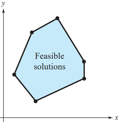
Figure 1: 2D Feasibility Region

The vertices of this region—where the lines of the constraints intersect—indicate the points (x, y) where the optimal solution can be found. This bounded area is known as a convex polytope, and in three dimensions, it would manifest as a closed volume:

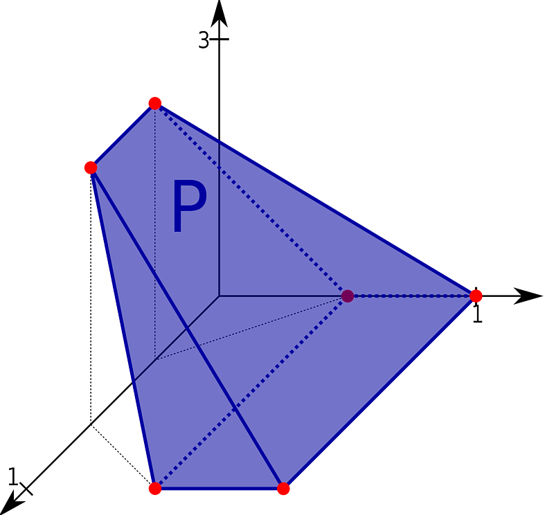
Figure 2: 3D Feasibility Region

It's important to note that the feasible region may not always be closed; in some cases, open problems exist where one side is unbounded, typically yielding either a minimum or maximum but not both. To tackle a linear programming (LP) problem, we first need to identify what the feasible region looks like. Take, for instance, the following LP problem:

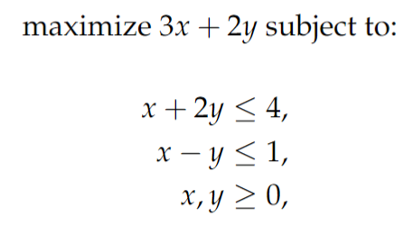
LP Problem 1

In this scenario, the function f(x, y) = 3x + 2y serves as our objective function, and our goal is to determine its maximum within the feasible region defined by the inequalities. We can illustrate this region by identifying the intersections of those linear inequalities:

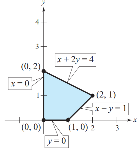
Figure 3: Feasible Region for LP Problem 1

Having identified the vertices of the convex polytope, we can evaluate f(x, y) at these points to ascertain the maximum value:

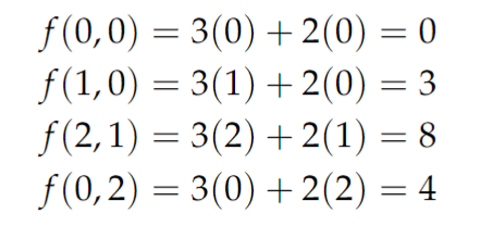
This process reveals that f(x, y) achieves a maximum value of 8 when x = 2 and y = 1. This graphical method is manageable with two variables, but for higher-dimensional LP problems, we must adopt a different approach. Here, we will implement the Python function linprog from the scipy.optimize module.

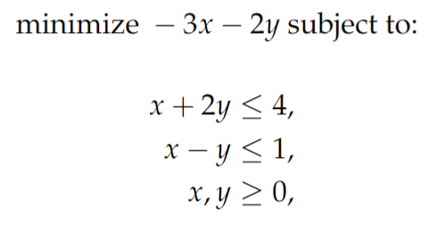
To utilize this function, we must first reformulate the linear program as a minimization problem instead of maximization. This involves multiplying the objective function by -1 and reversing all inequality signs, ensuring they point in the desired direction. The two constraints can remain unchanged as they explicitly define the bounds for both variables. The reformulated program appears as follows:

LP Problem 2

This adjustment retains the same problem structure, with the only change being the objective function's sign. Next, we express the bounds (x ≥ 0 and y ≥ 0) as tuples representing minimum and maximum values:

x_bounds = (0, None)

y_bounds = (0, None)

Here, None implies an open bound (infinity). The other two constraints can be arranged in a left-hand side matrix, denoted as A, and the right-hand side as vector b:

A = [[1, 2], [1, -1]]

b = [4, 1]

The coefficients of the cost function will be stored in a list, c:

c = [-3, -2]

Finally, we call the linprog function as follows:

sols = linprog(c, A_ub=A, b_ub=b, bounds=[x_bounds, y_bounds])

When we compile all these components into a single script, it looks like this:

from scipy.optimize import linprog

# Input parameters

x_bounds = (0, None)

y_bounds = (0, None)

A = [[1, 2], [1, -1]]

b = [4, 1]

c = [-3, -2]

# Solve problem

sols = linprog(c, A_ub=A, b_ub=b, bounds=[x_bounds, y_bounds])

print(sols.fun)

print(sols.x)

This results in the following output:

-7.999999999995814

[2. 1.]

The first line indicates the minimum value of the function, which is nearly -8. However, since we aimed to maximize f(x, y), we conclude that the maximum value of the original objective function f(x, y) = 3x + 2y is -(-8) = +8, occurring at the vertex (2, 1), which aligns with the values we calculated manually.

Although this example is straightforward, the linprog function can efficiently handle more complex LP problems with multiple variables, making it an invaluable tool for addressing linear optimization challenges.