Creating Custom Maps by Merging Polygons with Geopandas
Written on
Chapter 1: Introduction to Custom Maps
Have you ever wanted to design personalized maps for your dashboard tools, like Power BI, Looker Studio, or Tableau? If that’s the case, you’re in for a treat today!
Geopandas stands out as a robust library that streamlines the process of handling geospatial data. One of its most beneficial features for data visualization is its ability to merge polygons to create tailored regions and maps. In this guide, I will walk you through how to combine polygons of various European countries using Geopandas to form four distinct European regions. Let’s embark on this journey together! 🌍
In my role as a Data Analyst, I frequently engage with geospatial data, and as you might expect, dashboards play a critical role in showcasing this information. A typical task involves creating customized maps that align with the geospatial regions of interest. For my project, I needed to divide Western Europe into four main areas: Northern Europe, Southern Europe, Central Europe, and Benelux.
But before we dive deeper, let’s clarify a fundamental concept: What is a Polygon?
A polygon, in simple terms, is defined by a collection of points that outline a geometric shape with a geographical location. This can be utilized to represent the boundaries of countries and regions.
Section 1.1: Understanding the Geopandas Library
Geopandas is a Python library designed to facilitate the manipulation of geospatial data. It merges the powerful capabilities of Pandas for DataFrames with Shapely for geometric data, offering geospatial operations with the familiar syntax of Pandas while enhancing its functionality for geometries and map creation.
These geometric functions are executed by Shapely, with Fiona handling file access and Matplotlib being used for plotting. This library has been invaluable to me over the past few months, particularly for generating regional boundaries represented as Polygons.
Section 1.2: Setting Up Your Environment
To begin, if you haven’t yet installed the Geopandas library, you can easily do so by executing the following pip command:
pip install geopandas
Next, we need to load the necessary libraries and files. To effectively work with Geopandas, you will need the polygons corresponding to your desired geographical areas. Numerous maps (country, regional, and subregional) are available in JSON format on GitHub, which I highly recommend exploring.
For my project, I will utilize a JSON file containing all the world’s countries. You can find this file on my GitHub repository.

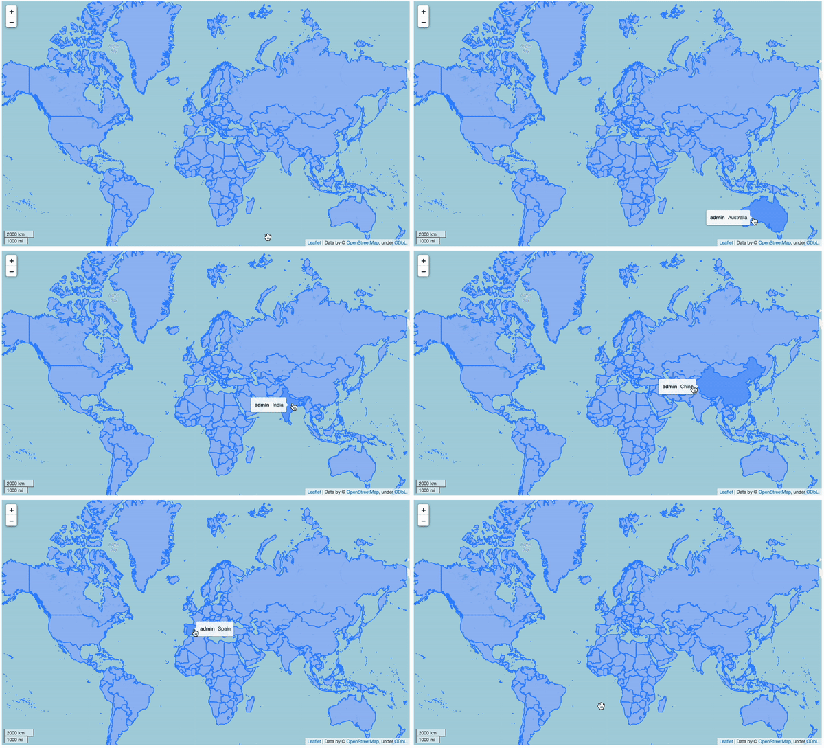
Using the exploration command, the regions under study are displayed on a map alongside all the information included in the DataFrame. However, my focus is on a specific list of European countries and their corresponding regions.
Chapter 2: Merging Polygons for Custom Regions
To merge the world map with the list of European regions, I will load a file that includes the country names, their ISO3 codes, and their respective European regions. You can find this file on my GitHub as well.
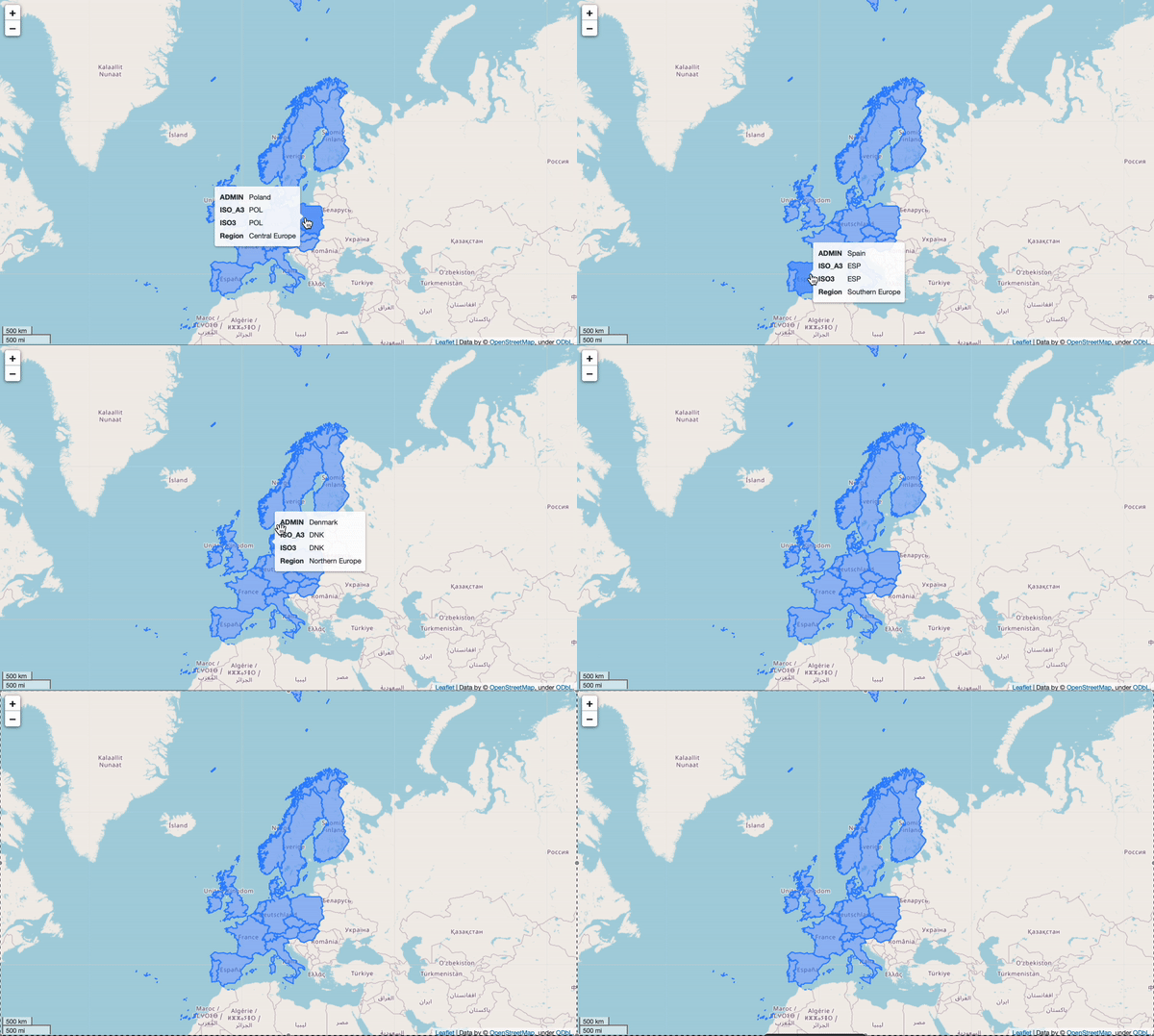
The Geopandas geometry map is as follows:

The newly created Geopandas DataFrame has four columns:
- The first column lists the country names.
- The second column contains the ISO3 codes.
- The third column includes the geospatial polygon for each country.
- The final column shows the corresponding European region for each country.
Section 2.1: Merging Multiple Polygons
The primary objective is to obtain the geometric boundaries of the four European regions. If we know which countries belong to each region, merging them becomes straightforward.
The shapely.ops library offers a function named cascaded_union, which allows for the combination of different polygons into one.
To achieve this, we need to define a function that returns the boundary of the combined polygons. I filter my Geopandas DataFrame to retain only those countries that belong to a specific region. For instance, I filtered all the countries included in the Southern Europe region.

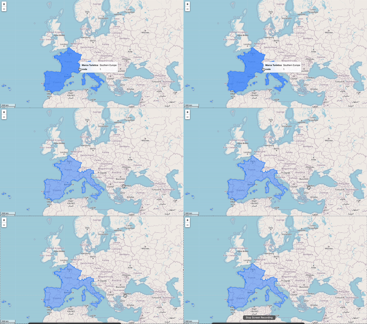
With the remaining subregion polygons, we can apply the unary_union command to merge them into a single polygon. This process will generate the corresponding map for the Southern Europe region.

Following this, we replicate the process for the other three regions. Once all the new polygons are created, a new DataFrame is generated, containing the geospatial polygon information for each of the four regions.
The DataFrame has three main columns:
- The name of the European region.
- The corresponding European region code.
- The geometry for each region.
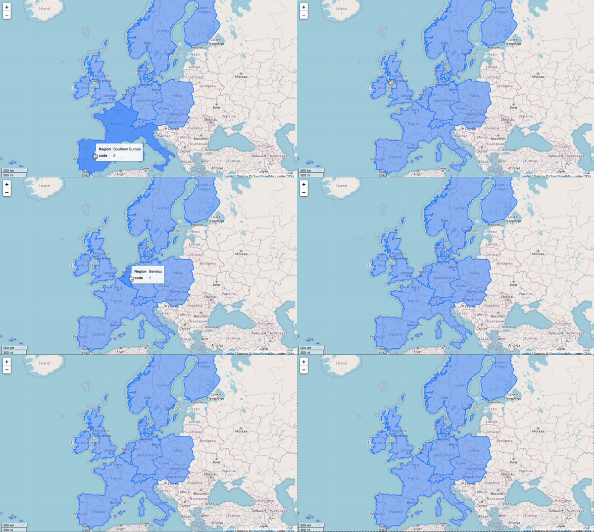
The final representation of the map looks like this:

And there you have it! We successfully created all four European regions!
In case you’re interested, my complete Jupyter notebook is available at the following link. I hope you find it easy to replicate!
Happy mapping! Don't forget to follow ForCode’Sake for more articles like this one!
The first video titled "Geopandas and Choropleths - Part 2: Merging Data" provides an in-depth guide on merging geospatial data using Geopandas.
The second video, "Create AMAZING Maps with Python! (GeoPandas Tutorial for Choropleth Maps)," showcases how to create stunning maps using Python and Geopandas.
Subscribe to my DataBites Newsletter to receive unique content directly in your inbox!
You can also connect with me on X, Threads, and LinkedIn, where I share daily insights on ML, SQL, Python, and Data Visualization.
Explore these related articles for further insights:
- What’s Behind Google Looker Studio — Unlocking the Power of Data Visualization
- Creating Your Own Dashboard Using Google Cloud Platform
- What’s Behind Elasticsearch? — Unlocking the Power of Data Visualization
- Creating a Google Looker Studio Dashboard — Populating it with Data